Database indexing is a data access technique that builds a separate, ordered lookup structure alongside a table so a query engine can find matching rows without scanning every row in the table. Oracle's own database concepts documentation defines an index as an optional structure, associated with a table or table cluster, that can sometimes speed data access, and that qualifier, sometimes, matters as much as the acceleration itself: an index is a targeted trade, faster reads on the columns it covers, in exchange for extra writes and storage on every column it touches. This article works through B-Tree, Hash, and composite/covering/partial indexes, the math that decides whether a given index is worth building, and the point where a query planner quietly ignores an index that exists.
What Database Indexing Does
Database indexing works by building a separate, ordered structure that points back to a table's rows, so a query engine can look up matching rows instead of reading every row in the table. PostgreSQL's own documentation states that by default, the CREATE INDEX command creates B-tree indexes, which fit the most common situations. Without an index, a query that filters on a column the engine has no lookup structure for forces a full table scan: read every row, evaluate the condition, discard what does not match. That cost is invisible on a table with a few hundred rows, but on a table with tens of millions of rows, a full table scan turns an instant query into one that visibly drags, because the database has no shortcut to skip rows it already knows will not match.
An index changes that by keeping a sorted or hashed copy of the indexed column's values, each entry paired with a pointer back to the row that owns it, narrowing the search dramatically before the engine touches the table's actual rows. That acceleration is not free: every index has to be updated whenever a row it covers is inserted, changed, or removed, and it occupies its own block of storage separate from the table. The database administrator (DBA), or the application team that owns the schema, decides which columns earn that ongoing cost against how urgently a query needs to skip a full table scan, a trade-off this article returns to after covering the three structures that implement it.
Indexing decisions look different depending on the workload. A transactional (OLTP) application, an order-processing system or a user-account service, needs indexes that keep individual lookups fast without slowing the constant stream of writes, while preserving the Atomicity, Consistency, Isolation, and Durability (ACID) guarantees an index touches on every write. An analytical (OLAP) workload scanning millions of rows for a report cares more about scan efficiency than single-row speed, which is why analytical engines often rely less on B-tree indexing altogether. IBM, Microsoft, and Oracle each ship general-purpose engines that support standard, ANSI SQL-based B-tree indexing across both workload shapes; NoSQL engines such as MongoDB and Cassandra implement their own index structures outside that relational lineage entirely.
B-Tree Indexes: The Default for a Reason
A B-tree index is a balanced, multi-way tree that keeps indexed values in sorted order, which is why it handles both exact-match and range queries well. PostgreSQL's documentation is direct about the mechanics: PostgreSQL includes an implementation of the standard btree (multi-way balanced tree) index data structure, and any data type that can be sorted into a well-defined linear order can be indexed by a btree index. Numbers, dates, and text all have that natural linear order, so a B-tree can arrange them into a tree where each lookup eliminates roughly half of the remaining candidates.
Oracle's own concepts documentation frames B-tree as the field's baseline structure: B-trees, short for balanced trees, are the most common type of database index, an ordered list of values divided into ranges that provides excellent retrieval performance for exact match and range searches. SQL Server adds its own vocabulary on the same structure: SQL Server rowstore indexes are described as either clustered or nonclustered B-tree indexes, and a clustered index sorts and stores the data rows of the table in order based on the clustered index key, SQL Server's own terminology for the same B-tree mechanics, not a universal vocabulary every engine shares.
- Equality lookups (WHERE user_id = 4821), where the tree narrows to one matching leaf quickly
- Range scans (WHERE created_at BETWEEN two dates, or WHERE price > 50), because sorted order lets the engine walk a contiguous slice of the tree
- Sorted-order retrieval (ORDER BY on the indexed column), since the tree is already in that order and the database can skip a separate sort step
- Prefix matching on text columns (WHERE last_name LIKE 'Jones%'), which behaves like a range scan over sorted string values
B-tree is the general-purpose default because it handles equality, range, and sort-order queries reasonably well at once. Hash indexes give up two of those three capabilities in exchange for being faster at the one they keep.
Hash Indexes: Faster Lookups, Narrower Use Case
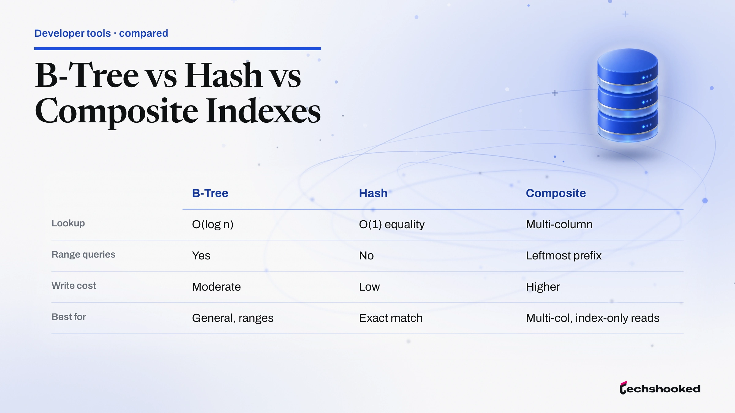
Database indexing has a second structure worth knowing beyond B-tree: the hash index. A hash index trades the B-tree's ordered structure for a hash table, which makes single-value equality lookups faster but drops support for range queries entirely. PostgreSQL states this contrast directly: B-trees can handle equality and range queries on data that can be sorted into some ordering, while hash indexes can only handle simple equality comparisons. A hash function maps each indexed value to a bucket, so an equality lookup jumps straight to the right bucket, but that same hashing throws away the value's relative order, exactly what a range query needs.
MySQL's own manual draws the same line: a MySQL B-tree index can be used for column comparisons in expressions that use the =, >, >=, <, <=, or BETWEEN operators, while hash indexes are used only for equality comparisons using = or <=>, described as very fast for that narrow case. That narrowness is why hash indexes see far less general-purpose adoption than B-tree; most application queries eventually need a range filter, a sort, or a prefix match, and a hash index cannot serve any of those.
| Capability | B-Tree Index | Hash Index |
|---|---|---|
| Equality lookup (=) | Supported | Supported, often faster for this case alone |
| Range query (BETWEEN, >, <) | Supported | Not supported |
| Sorted-order retrieval | Supported (already ordered) | Not supported |
| Typical use case | General-purpose default | Narrow, equality-only lookup tables |
| Default index type | PostgreSQL, Oracle, MySQL, and SQL Server all default CREATE INDEX to B-tree | Available as an explicit option, not a default, in PostgreSQL and MySQL |
A hash index is worth reaching for only when a workload is genuinely, permanently equality-only, a lookup table keyed by a fixed identifier with no range or sort requirement ever appearing in production. Outside that narrow shape, the B-tree's broader coverage usually wins even if a hash index would theoretically be faster for the one pattern it supports, which is why B-tree stays the default in Postgres, Oracle, and SQL Server alike. Key-value stores such as Redis and Cassandra lean far more heavily on hash-style lookups, since their workloads are equality-only by design.
Composite, Covering, and Partial Indexes
Database indexing is not limited to a single column. A composite index extends the same B-tree mechanics across more than one column, and Oracle's documentation defines it precisely: a composite index, also called a concatenated index, is an index on multiple columns in a table, one that can speed retrieval for SELECT statements whose WHERE clause references all or the leading portion of the composite index's columns, and the order of those columns matters: the most commonly accessed ones go first. PostgreSQL's multicolumn guidance reinforces the same point: an index can be defined on more than one column of a table, usable with query conditions on any subset of its columns, but most efficient with constraints on the leading, or leftmost, columns.
Covering and partial indexes narrow the same idea further, in two different directions.
- Composite index: a single B-tree index built across two or more columns, most efficient when a query filters on the leading column, the leftmost column of the index definition, per both the Oracle and PostgreSQL guidance above. Column order should follow how queries actually filter: equality columns first, range-filtered columns last. A composite index on (customer_id, order_date) for an orders table serves queries filtering on customer_id, alone or with order_date, but not one filtering on order_date alone, since customer_id is the leading column, the exact shape of order-processing systems at Amazon, Shopify, or Stripe.
- Covering index: an index that includes enough columns to answer a query entirely from the index structure itself, so the engine never needs a separate lookup back to the table row. SQL Server's own documentation on indexes with included columns describes exactly this mechanism, adding extra columns to an index specifically so a query can be satisfied without touching the base table. A covering index on (email, first_name, last_name) lets a login page render a user's display name straight from the index, a pattern common in applications built on Laravel, Spring Boot, or Express.
- Partial index: an index built over a filtered subset of a table's rows rather than every row, useful when queries consistently filter on a condition that only matches a small fraction of the table, for example an index that only covers rows where a status column equals one specific, narrow value. This keeps the index small and its write cost limited to the rows it actually covers, at the cost of being useless for any query outside that filtered subset.
A wider or more specific index is not automatically better: a composite index with the wrong column order, a covering index with columns no query needs, or a partial index whose filter misses real query patterns all pay the same write and storage cost as a well-designed one, without the same read benefit.
B-tree, hash, and composite indexes cover most application queries, but PostgreSQL's own documentation lists several specialized structures built for narrower data shapes: GIN (Generalized Inverted Index) for values containing multiple components, such as arrays, and BRIN (Block Range Index) for summarizing values across consecutive physical block ranges of a large table. GiST and SP-GiST round out PostgreSQL's index method list for geometric and hierarchical data shapes that neither B-tree nor hash handle well, and dedicated search engines such as Elastic, Solr, and the underlying Lucene library build their own inverted-index structures for tokenized full-text search rather than extending a B-tree or GIN index to the task. No single index structure, B-tree included, is the right tool for every data shape a database has to store.
Most applications never write CREATE INDEX by hand. Django, Ruby on Rails, Hibernate, Symfony, and Laminas all generate index definitions from model annotations, though the underlying B-tree, hash, or composite structure the database actually builds is identical either way. That holds on managed hardware too: Amazon RDS, Google Cloud SQL, and Azure SQL Database from Amazon Web Services, Google Cloud, and Microsoft Azure, plus smaller providers like Digital Ocean, Heroku, and Supabase, all run the same PostgreSQL, MySQL, and SQL Server engines underneath a managed control plane, alongside enterprise engines such as IBM Db2, Sybase, Informix, and SAP HANA and newer cloud-native entrants like Neon, PlanetScale, and Timescale. Choosing a provider changes who patches the server, not which index structures are available.
Selectivity, Cardinality, and the Write-Amplification Trade-off
Index selectivity measures what fraction of a table's rows a given predicate eliminates, the single biggest factor in whether an index actually helps a query. Selectivity is tied to cardinality, the number of distinct values a column holds relative to the table's row count. A high-cardinality equality filter, a user ID, an email address, an order number, is highly selective: an index on it eliminates almost everything else immediately. A low-cardinality filter, a boolean flag, a status field with three possible values, is poorly selective, and an index on it alone rarely beats a full table scan for anything but a genuinely rare value. A country column illustrates the point directly: an index on country helps a query for a small country like Iceland or Luxembourg far more than one for a large country like India or the United States, where a single value can still match millions of rows.
Index selectivity decides whether an index helps a read. Write amplification is the cost side of the same trade, and it applies regardless of how selective the indexed column is.
- Every index a database maintains must be updated on every insert, update, or delete that touches an indexed column, a write amplification cost that is the direct price of the index existing at all.
- Each index consumes its own storage, separate from the table's own data, so a heavily indexed table can end up with a combined index footprint that exceeds the size of the table it indexes.
- More indexes give the query planner more options to weigh during planning, adding a small amount of planning overhead, though this cost is minor compared to the ongoing write cost above.
- The practical trade-off favors fewer, well-chosen indexes on genuinely high-selectivity columns that queries actually filter on, not indexing every column defensively on the chance a future query might need it.
This is the direct counterweight to treating indexing as a pure win: an index on a low-cardinality column pays its write and storage cost on every write forever, whether or not it ever earns that cost back on a read. The database's query planner ultimately decides whether an index gets used at all, which is where a poorly targeted index stops being merely inefficient and starts being dead weight. The storage medium underneath matters too: an SSD or NVMe drive absorbs an index's extra random writes far better than a spinning HDD, since solid-state storage skips the mechanical seek penalty that made index-heavy writes expensive on older hardware. IOPS capacity, not just storage space, is part of the real budget an index consumes.
How the Query Planner Decides to Use an Index
Database indexing decisions do not end once a structure is built; the query planner has the final say on whether it gets used, weighing the cost of an index lookup against a full table scan and picking whichever plan it predicts will be cheaper for that specific query.
- The planner relies on table and column statistics, row counts, value distribution, cardinality estimates, so stale statistics after a large data load can cause it to underestimate an index's benefit and skip it even when the index would genuinely help.
- A composite index is generally only usable by the planner when the query's WHERE clause constrains its leading column, the leftmost column in the index definition, the same behavior PostgreSQL's own multicolumn documentation describes: efficiency depends on constraints on the leading columns. A query that only filters on a trailing column of a composite index typically cannot use that index efficiently at all.
- For a low-selectivity predicate that would match a large fraction of a table's rows, the planner often chooses a full table scan over an index lookup, because reading the whole table sequentially can be cheaper than following many scattered index pointers back to individual rows one at a time.
- Wrapping an indexed column in a function call or type cast inside a WHERE clause commonly prevents the planner from using a standard index at all, since the index stores raw column values, not the output of a function applied to them.
- Column-oriented analytical engines such as Snowflake, Databricks, and Amazon Redshift lean on scanning compressed column chunks rather than row-level B-tree indexes for most queries, since indexing strategy depends on whether the underlying engine is row-oriented or column-oriented.
An index the planner will never choose for the query shapes actually running pays its full write and storage cost for zero read benefit, the practical answer to when not to index a column. That is a distinct question from how an entire dataset gets distributed across machines in the first place, a cross-node concern handled by choosing between PostgreSQL, MongoDB, and Redis and by horizontal partitioning strategies more broadly. Indexing stays entirely within one database node, accelerating how fast that node finds rows it already stores; which node stores which rows is a separate architectural decision, and query planner behavior and index defaults differ by engine.
Teams that get this far often also have to decide how the services querying that database talk to each other, particularly once gRPC, REST, and message queues enter the picture as separate services share the same well-indexed tables, and how query results reach a browser once they come back fast, whether through a simple request-response cycle or a persistent channel like WebSockets or Server-Sent Events. Indexing solves the lookup half of that pipeline; everything downstream is a separate set of trade-offs.
References
- Index Types, PostgreSQL Documentation
- B-Tree Indexes, PostgreSQL Documentation
- Multicolumn Indexes, PostgreSQL Documentation
- Indexes and Index-Organized Tables, Oracle Database 19c Database Concepts
- Indexes and Index-Organized Tables, Oracle Database 18c Database Concepts
- CREATE INDEX, Oracle Database 19c SQL Language Reference
- SQL Server and Azure SQL Indexes, Microsoft Learn
- CREATE INDEX (Transact-SQL), Microsoft Learn
- Create Indexes with Included Columns, Microsoft Learn
- Comparison of B-Tree and Hash Indexes, MySQL Reference Manual
Further reading
Frequently Asked Questions
Does adding more indexes always make queries faster?
No. Every index a database maintains adds write cost on every insert, update, or delete that touches an indexed column, plus its own separate storage footprint, so an index on a rarely-queried or low-selectivity column can cost more than it saves. The query planner also has to consider more options during planning as index count grows, though that overhead is small compared to the write cost. The right number of indexes is the smallest set that covers the queries actually running against a table, not the largest set that could theoretically help.
Why would a database skip an index and scan the whole table instead?
The query planner estimates the cost of using an index against the cost of a full table scan and picks whichever it predicts is cheaper. For a predicate that matches a large fraction of a table's rows, a low-selectivity filter, sequentially reading every row can be cheaper than following many scattered index pointers back to individual rows, so the planner deliberately chooses the scan. Stale table statistics after a large data load can also cause the planner to underestimate an index's benefit and skip it.
Does column order matter in a composite index?
Yes. PostgreSQL's own documentation states a multicolumn B-tree index is most efficient when queries constrain the leading, or leftmost, columns, and Oracle's documentation makes the same point directly: the order of columns in a composite index is important, and the most commonly accessed columns should go first. A query that only filters on a trailing column of a composite index typically cannot use that index efficiently, so column order should follow how queries actually filter, not the order columns happen to appear in the table.
When should a column not be indexed at all?
A low-cardinality column, one with few distinct values relative to the table's row count, is a poor indexing candidate. A column that is rarely used in a WHERE clause, JOIN condition, or ORDER BY is also a weak candidate, because the write and storage cost of maintaining its index is paid on every write regardless of whether the index ever helps a read. Small tables are another case: when a full table scan is already fast because the table itself is small, an index adds overhead without a meaningful read-speed benefit.