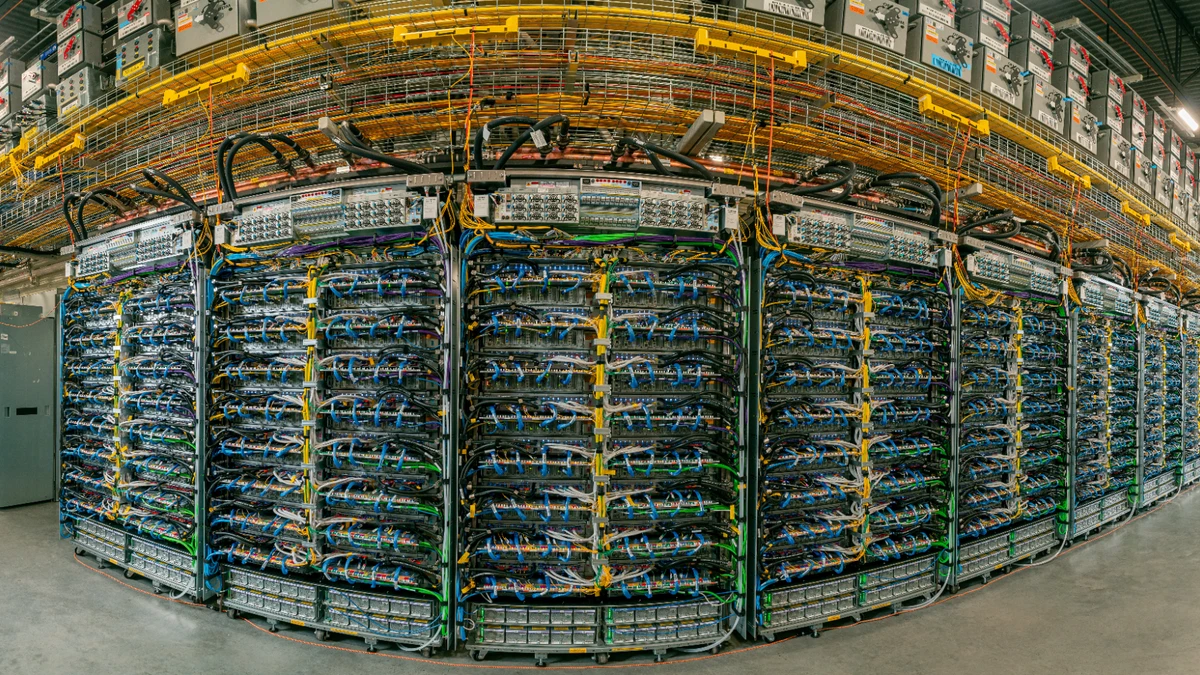
Inference cost is the price that an operator pays each time a model generates output, driven by token volume, model size, hardware, and the serving strategy chosen to balance throughput against latency. Hosted APIs from OpenAI, Anthropic, and Google Cloud surface this as a per-token rate; teams running their own NVIDIA H100 or A100 fleets see it as GPU-hours, memory bandwidth pressure, and KV cache occupancy. The two views describe the same underlying physics: floating point operations consumed per generated token, multiplied by the rate at which the GPU can move weights from high-bandwidth memory through its compute units. Every cost-reduction lever, from batching to quantization to KV cache reuse, manipulates one of those variables. Understanding which lever applies to which workload is the difference between a roughly $0.01-per-call assistant and a runaway monthly bill. The mechanics also explain why two models with similar capability can sit at very different price points, and why the same model can vary by an order of magnitude in cost depending on how it is served. For the wider serving picture, see how AI models are served at scale.
What Inference Cost Actually Measures

Inference cost measures the compute resources consumed each time a model processes an input and produces an output, expressed in dollars per token on hosted APIs or in GPU-hours per request on self-hosted deployments. The metric collapses several distinct quantities into one number: floating point operations (FLOPS) executed by the GPU, bytes moved between high-bandwidth memory (HBM) and the compute cores, the wall-clock time the request occupied an accelerator, and the share of fixed serving overhead that the request absorbed. OpenAI exposes the simplest version of this on its public pricing page, where each model carries an input token rate and a separate output token rate (OpenAI API Pricing). Google Cloud's Gemini pricing separates input and output rates, with audio tokens carrying a distinct rate on some model variants and cached input billed at a fraction of the standard input rate; exact figures vary by model family (Google Cloud Generative AI Pricing). Self-hosted operators read the same quantity differently: a request that takes 200 milliseconds on a rented H100 instance has a marginal cost equal to the hourly rate times the fraction of an hour consumed, adjusted for the GPU utilization actually achieved. Both views matter, and conflating them is the most common budgeting mistake teams make.
- Inference cost: the marginal price of one model call, billed in tokens on hosted APIs or computed from GPU-hours on self-hosted infrastructure.
- Token: the unit a model reads and writes, usually a word fragment of two to four characters; both prompt and output tokens incur compute.
- FLOPS: floating point operations per second, the throughput measure for raw compute on a GPU such as the NVIDIA H100 or A100.
- HBM: high-bandwidth memory on the GPU, where model weights and the KV cache sit during a forward pass.
- Utilization: the fraction of GPU compute and memory actually doing useful work during a request; idle silicon still costs full hourly rate.
How Token Volume and Context Window Length Drive Cost
Inference cost scales directly with token count because every token a model reads or writes requires a forward pass through some portion of the network, and longer context windows compound this by increasing the KV cache the GPU must hold in memory. A request with a long multi-thousand-token prompt and a short output triggers many times the input-side compute of an equivalent short prompt, because every prompt token flows through the attention layers before the first output token is generated. Output tokens are typically priced higher than input tokens on hosted APIs, reflecting that each generated token also triggers autoregressive decoding that reads back through the entire context. The Google Cloud pricing page for Gemini lists separate input and output rates, with audio tokens billed at a distinct rate on some model variants and a discounted cached-input rate available across the family (Google Cloud Generative AI Pricing). Context window length amplifies the effect in two ways. Memory pressure rises because the KV cache for a long context can dominate HBM usage, cutting the batch size the GPU can hold and lowering tokens per second (TPS) across all concurrent users. Attention compute also scales quadratically with sequence length in the naive case, though modern serving stacks such as vLLM and TensorRT-LLM use FlashAttention and paged KV caching to soften the curve. Teams that drop unused chat history, summarize older turns, or retrieve only the relevant snippets see token bills fall in lockstep with the trimming.
| Token type | What it covers | Typical pricing relationship | Workload lever |
|---|---|---|---|
| Input (prompt) | Every token in the prompt, system message, and retrieved context | Lowest per-token rate of the three on most APIs | Trim history, retrieve narrowly, share prefixes for caching |
| Output (completion) | Each token the model generates in the response | Typically several times the input rate on most vendors | Constrain response length, stop sequences, structured output |
| Cached input | Prompt prefix matched against a prior request and served from KV cache | Discounted to a fraction of the standard input rate | Stabilize system prompts so they hit the cache |
| Multimodal (image, audio) | Non-text inputs expanded into token-equivalents by the model | Billed per image or per second of audio, often translated to tokens | Downsample images, transcribe before sending audio |
Model Size, Memory Bandwidth, and Why Bigger Models Cost More

Inference cost rises with model size because a larger model requires more FLOPS per generated token and demands more GPU memory to hold its weights and activations resident during a forward pass. A 7-billion-parameter model in FP16 occupies roughly 14 GB of HBM for weights alone, fitting comfortably on a single NVIDIA A100 with 40 GB or 80 GB and leaving room for sizable batches. A 70-billion-parameter model in the same precision needs about 140 GB just for weights, which forces tensor-parallel sharding across two or more H100 GPUs and immediately doubles the hardware footprint per request. Memory bandwidth, not raw FLOPS, is often the binding constraint: autoregressive decoding reads the entire weight set from HBM for every generated token, so a model that fits in HBM with headroom decodes far faster than one that saturates it. VMware's LLM inference sizing guidance walks through this in detail, noting that memory bandwidth and capacity dominate inference performance for large autoregressive models far more than peak FLOPS does (VMware, LLM Inference Sizing and Performance Guidance). The practical consequence is that doubling parameter count rarely doubles cost; it often more than doubles, because the larger model also collapses the batch size the GPU can sustain. Teams that match model size to task, using a 7B or 13B for classification and routing while reserving a 70B class model for the genuinely hard requests, capture the largest cost wins available before any other optimization. For the silicon side of the trade-off, see how NPUs, GPUs, and TPUs differ for AI workloads.
- Pick the smallest model that clears the quality bar. Route easy requests to a 7B or 13B and escalate to a 70B class model only when scoring flags low confidence.
- Match precision to hardware. FP16 fits more on an A100; FP8 on an H100 nearly doubles effective HBM headroom without retraining for many checkpoints.
- Check memory bandwidth before FLOPS. Decoding throughput is gated by HBM bandwidth on large models; a chip with more TFLOPS but slower HBM can run slower in practice.
- Watch the batch-size cliff. A model that just fits leaves no room for batching, so per-token cost rises sharply versus one with comfortable headroom.
- Benchmark on realistic prompt and output lengths. Throughput curves bend at the lengths your traffic actually uses, not at the vendor's headline number.
Batching, Throughput, and the Latency Trade-off
Inference cost per request falls as batching increases throughput, since grouping multiple requests into a single forward pass amortizes weight-loading overhead across more tokens, but aggressive batching lengthens queue time and degrades latency for individual users. Static batching, the older approach, waits until a fixed number of requests arrive and then runs them together; the slowest request in the batch sets the response time for everyone in it. Continuous batching, popularized by the vLLM serving stack and adopted in TensorRT-LLM and Hugging Face's TGI, instead schedules at the token step level. New requests join a running batch on any decoding step, and finished requests leave without waiting for the slowest peer. Databricks documents the throughput gain with a concrete figure: continuous batching can deliver "10x-20x better throughput than dynamic batching" by keeping the GPU saturated even when individual request lengths vary widely (Databricks, LLM Inference Performance Engineering Best Practices). The trade-off is unavoidable, though. A single low-latency request served alone on a GPU pays the full weight-loading cost itself and produces high tokens per second for that user, at the price of a near-empty GPU. A batch of 32 requests divides that overhead by 32 but adds wait time as the scheduler holds slots open. The cost-optimal operating point depends on the workload's latency budget: chat assistants tolerate 200-300 ms time-to-first-token and accept aggressive batching, while real-time voice agents cap at 100 ms and pay more per call to hit it.
- Continuous batching first. Move off static batching to vLLM or TensorRT-LLM; the throughput gain is usually multiples without code changes upstream.
- Separate latency tiers. Route interactive traffic and background batch jobs to different endpoints so one does not starve the other.
- Tune max batch size to HBM headroom. Set the cap so the worst-case KV cache plus weights still fits with margin, not at the theoretical maximum.
- Track TPS per GPU, not just per request. The cost-revealing metric is aggregate tokens per second the GPU sustains, not the speed any single user sees.
- Consider managed scaling. Cloud-native platforms handle autoscaling and continuous batching for you; for context, see managed ML platforms that handle inference scaling.
KV Cache, Quantization, and Cost Reduction Techniques
Inference cost can be reduced substantially through caching and compression: KV cache reuse eliminates redundant computation for shared prompt prefixes, while quantization shrinks weight precision from FP16 to INT8 or INT4, fitting larger models onto fewer GPUs. The KV cache stores the key and value tensors produced by attention for every token already processed, so the model never recomputes them when generating the next token. Prefix caching takes this further: when many requests share a common system prompt or retrieved document, the cached KV state for the shared portion serves all of them, and only the unique tail of each request consumes fresh compute. Shared prefixes are common in agent workloads, code assistants, and retrieval-augmented chat, which makes prefix reuse one of the higher-impact interventions available to production LLM serving stacks such as vLLM and TensorRT-LLM. Anthropic and OpenAI both expose cached-input pricing as a discount on the standard input token rate, recognizing the genuine compute saving. Quantization attacks a different axis. Dropping weights from 16-bit to 8-bit halves HBM occupancy and roughly doubles the model size that fits on a given GPU; INT4 quantization, used by tools such as TensorRT-LLM and llama.cpp, halves it again, with measured quality drops typically small on well-tuned checkpoints. Speculative decoding pairs a small draft model with the target model, letting the target verify several speculative tokens in parallel and producing throughput gains when the draft model agrees often.
- Prefix caching: reuse the KV cache for shared system prompts and retrieved context across requests; supported in vLLM, TensorRT-LLM, and the major hosted APIs.
- INT8 quantization: halves weight memory versus FP16, doubles effective HBM headroom, and typically holds quality on instruction-tuned models.
- INT4 quantization: halves it again; suitable for batch and offline workloads where small quality regressions are tolerable.
- Speculative decoding: a small draft model proposes tokens that the target model verifies in parallel; effective when the draft agrees often.
- Distillation and routing: train a smaller model to mimic a larger one for the common case, and escalate only when scoring flags uncertainty.
- Stop sequences and structured output: cap output token counts directly at the API; the cheapest token is the one never generated.
Hosted API Pricing vs. Self-Hosted Infrastructure Math
Inference cost looks very different depending on whether you read it from a vendor's API pricing page or compute it from your own GPU utilization, and conflating the two is one of the most common mistakes teams make when budgeting AI workloads. Hosted APIs from OpenAI, Anthropic, and Google Cloud bill per token at a published rate, with the vendor absorbing the GPU fleet, batching, scaling, redundancy, and uptime obligations behind that rate (OpenAI API Pricing). The price is genuinely all-in for the operator's purposes, but it includes the vendor's margin and the cost of idle capacity reserved to absorb traffic spikes. Anthropic offers two service tiers, Standard (the default) and Priority (committed capacity for higher availability), which shape rate-limit behavior and pricing for synchronous traffic (Anthropic API Service Tiers). Separately, Anthropic's Message Batches API provides a discounted asynchronous path for offline workloads in exchange for slower turnaround, so high-volume batch traffic can drop the effective per-token bill substantially. Self-hosted economics invert the picture. The hourly rate of a rented H100 instance is fixed regardless of how many tokens flow through it; the per-token cost falls as utilization rises and balloons when the GPU sits idle. A team running a poorly-utilized fleet often pays more per token than the hosted API for the same model, while a team holding sustained 70-80% utilization on a continuous-batching stack can land below it. Rate limits matter on both sides. Hosted APIs cap requests per minute and tokens per minute per account tier, so practical throughput can fall below the per-token math suggests, while self-hosted operators set their own caps and pay the over-provisioning cost directly. For the broader operational picture, including how teams monitor and right-size these deployments, see deploying and monitoring AI in production with LLMOps.
| Dimension | Hosted API (OpenAI, Anthropic, Google Cloud) | Self-hosted (rented or owned GPU fleet) |
|---|---|---|
| Pricing unit | Per input and output token, with cached-input discounts | Per GPU-hour, regardless of token throughput achieved |
| Headline rate visibility | Public pricing page, updated by vendor | Cloud provider hourly rate; effective per-token rate depends on utilization |
| Operational overhead | Vendor handles batching, scaling, failover | Operator runs vLLM or TensorRT-LLM, autoscaling, monitoring |
| Throughput ceiling | Rate limits per account tier; Anthropic Standard and Priority shape it, Batch API runs offline | Limited by purchased GPU count and serving stack efficiency |
| Cost levers | Smaller models, Batch API, prefix caching, output limits | Quantization, continuous batching, utilization, GPU choice |
| Break-even | Predictable at any scale; margin baked into rate | Lower at high sustained utilization; worse at bursty or low traffic |
References
- OpenAI, API Pricing
- Anthropic, API Service Tiers
- Google Cloud, Generative AI Pricing
- Databricks, LLM Inference Performance Engineering Best Practices
- VMware, LLM Inference Sizing and Performance Guidance
Further reading
Frequently Asked Questions
What is the single biggest driver of AI inference cost?
Token volume is the single biggest driver of inference cost in hosted API billing. Every token the model reads (prompt) or writes (output) incurs compute; a request with a long multi-thousand-token prompt costs many times more than an equivalent short prompt with the same output, because the model must process every input token through its attention layers before generating any output.
Why does a larger model cost more to run than a smaller one?
A larger model requires more floating point operations per generated token and more GPU memory to hold its weights resident. An NVIDIA H100 GPU can serve a 7-billion-parameter model at far higher throughput than a 70-billion-parameter model on the same hardware, because the smaller model's weights fit in high-bandwidth memory with room for large batches, while the larger model saturates available VRAM and cuts batch size.
Does batching always reduce inference cost?
Batching reduces cost per token by spreading weight-loading overhead across more requests in parallel, but it does not always reduce cost for every user. Larger batch sizes improve GPU utilization and throughput, yet they also lengthen queue wait time, so a system optimized for throughput may produce worse latency than one provisioned for low response time at the expense of higher per-token cost.
What is KV cache and how does it reduce inference cost?
KV cache stores the key and value tensors computed for each token in the context so the model does not recompute them on subsequent generation steps. For requests that share a common system prompt or prefix, prefix caching lets multiple users reuse the same stored KV state, eliminating redundant compute for the shared portion and lowering the effective cost per request in high-volume deployments.